HabiCAT 3D

Habitat Complexity Analysis Tool 3D

HabiCAT 3D is an open-source application for visualizing, analyzing, and annotating the products of Structure-from-Motion (SfM) photogrammetry (meshes, point clouds, camera poses, and source photos) in a single, fully 3D environment. It implements novel algorithms for generating multi-scale complexity metrics maps (like rugosity, fractal dimension, vector dispersion and others) that capture the full three-dimensional complexity of real-world environments, including overlapping features such as branching corals that 2.5D approaches miss. Designed for ecologists and researchers, this tool is aimed at coral reefs and other complex structures, and also works with other 3D data such as topobathy lidar.

» Download HabiCAT 3D «

     (version 0.9.1 – September 21, 2026)

» Download Sample Models «

» Quick start guide for GUI mode «

» Quick start guide for CLI mode «

Features

• Meshes and Point Clouds: Several meshes and point clouds can be loaded into one scene as analysis objects. Each object keeps its own set of layers, and objects can be shown together or individually, so results computed on a point cloud can be viewed in the context of the mesh.
  • Supported formats: OBJ and PLY meshes; PLY, LAS and LAZ point clouds.
• Multi-Scale Maps: Generates detailed maps over varying scales to capture the intricate details of complex models.
• Complexity Metrics Available to Calculate:
  • On meshes:
    • Rugosity:
      • Average Normal(default): The simplest and fastest way to calculate rugosity, but for more acurate results, we highly recommend using “Min Rugosity”.
      • Optimized Reference Planes(Min Rugosity): A rugosity-minimizing technique for accurate reference plane selection, improving calculation accuracy.
      • Unique Projected Area: To correctly calculate rugosity on very complex models, users can opt to use this option. Currently, it is very slow, but we plan to improve its performance in the future.
    • Fractal Dimension.
    • Vector Dispersion.
    • Triangle Area.
    • Triangle Density.
  • On point clouds:
    • Point Density.
    • Fractal Dimension.
    • Structural Roughness.
• Layers: Our layer system allows users to compare results obtained using different metrics and settings. Each analysis run creates a new layer, which can be accessed through tabs at the top of the screen. Users can visually compare layers or generate heatmaps to highlight the differences between them.
  • Interpolation Layer (experimental): Interpolates between existing layers selected by the user. For example, after calculating the same metric at several voxel sizes, a slider moves through the interpolated results, which helps with choosing the size at which features of interest stand out.

• Camera Poses and Source Photos: Load a COLMAP-format reconstruction folder (cameras, images, optionally tie points, and the photos folder).
  • Camera positions are shown in the scene. Selecting one displays its frustum and pose information, and its original photo can be opened with the “Show original Photo” button.
  • Select triangles on a mesh to highlight the photos that should contain them.
  • Render the scene from any camera’s exact pose for comparison with the source photo.
• Annotations:
  • Import: Polygon annotations from vector files (.shp, .gpkg, .geojson) can be applied to meshes and point clouds.
  • VR annotation (experimental): A spherical cursor labels triangles or points directly in 3D. This is useful for fixing 2D annotations that project onto the wrong surface, e.g. the seafloor under a coral.
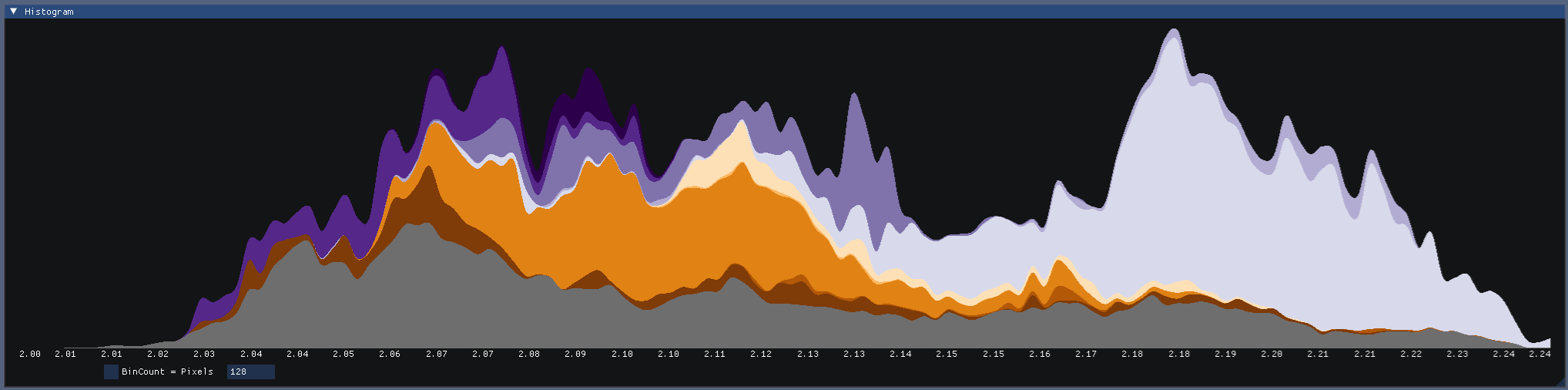
  • Stacked histograms: Show how each annotation class is distributed across complexity values (by surface area for meshes, by point count for point clouds).
    

• .RUG file format: Users can save and load entire workspace using a custom (.RUG) format. RUG files save all loaded objects together with their layers, decreasing load times and eliminating the need to re-run calculations.

• Histograms: Interactive histograms provide deeper insight into the distribution of complexity metrics across the model. At a glance, it is possible to quickly evaluate the uniformity or concentration of complexity in a model.

  • Histogram selection: Histograms can be queried by mouse to calculate how much surface area falls within a complexity range. Regions corresponding to selected ranges are highlighted to aid correlating the histogram to the model:

• CLI Scripting: The application supports a command-line interface (CLI) and script execution without a graphical user interface (GUI), allowing for streamlined integration into existing researchers’ workflows.

• Export Options:

  • Selection tool (Only in GUI Mode): The user can query the layer value of a single triangle or the layer values within a specified radius of a point. If the ‘Export to File’ option is activated, then the values will be automatically saved to a text file.
  • Screenshot (Only in GUI Mode): The ‘Take Screenshot’ button generates a screenshot without the GUI and with a larger legend, making it suitable for use in figures.
  • Whole Layer as Image: Layer values will be projected onto a plane and converted to a PNG or GeoTIFF (color or 32-bit float with raw values) image. The 32-bit float raw export is essential for easy use of the application’s calculation results in other applications.
    • Cumulative Suboption: In complex 3D models, multiple triangles may project to the same pixel when creating a 2D image. The cumulative option resolves this by accumulating the complexity metric along the projection axis, creating an “X-ray” effect that preserves information about high-complexity areas. This option is useful for models with overhangs and caves. ## Quick Start Guides

Quick start guide for GUI mode.

Quick start guide for CLI mode.

How To Get

• Download ready-to-use application: Latest release
• Download source code and compile: Look for instructions below.

How to compile

» Visit the HabiCAT 3D Repository «

The compilation process was tested with Windows 10 (and 11) and Visual Studio 2026. To compile, you would need Git, CMake, and Visual Studio.

# Initialize a new Git repository
git init

# Add the remote repository
git remote add origin https://github.com/Azzinoth/HabiCAT3D

# Pull the contents of the remote repository
git pull origin master

# Initialize and update submodules
git submodule update --init --recursive

# Generate the build files using CMake
# CMake should be added to a PATH
# if not then use CMAKE GUI
cmake CMakeLists.txt

After running these commands, you should have a Visual Studio project that is ready to be compiled.

Citing this work

Paper link: https://www.frontiersin.org/journals/marine-science/articles/10.3389/fmars.2025.1449332

If you use this code in your research, please cite:

K. Beregovyi and T. Butkiewicz, "HabiCAT 3D: Unified Visualization, Analysis, and Annotation of Structure-from-Motion Scans" in OCEANS 2026, 2026.

K. Beregovyi, J. Dijkstra and T. Butkiewicz, “Calculating 3D rugosity maps for complex habitat scans,” Frontiers in Marine Science, vol. 12, 2025.

Acknowledgements

This research was made possible through the support of NOAA Grants NA20NOS4000196 and NA25NOSX400C0001.

This is a project of Data Visualization Research Lab within the Center for Coastal and Ocean Mapping at the University of New Hampshire.

Third Party Licenses

This project uses the following third-party libraries:

1. Focal Engine: This library is licensed under MIT License. The full license text can be found at Focal Engine’s GitHub repository
2. CGAL: Some parts of CGAL are available under the LGPL, whereas other parts are under the GPL. The full license text can be found at CGAL’s GitHub repository or CGAL’s webpage.
3. boost: This library is licensed under Boost Software License. The full license text can be found at boost’s GitHub repository
4. Eigen: This library is part of CGAL.
5. GDAL: This library is licensed under MIT License. The full license text can be found at GDAL’s GitHub repository
6. FESceneGraphUI: This library is licensed under MIT License. The full license text can be found at FESceneGraphUI’s GitHub repository
7. LASzip: This library is licensed under Apache License 2.0. The full license text can be found at LASzip’s GitHub repository